An implementation of the SAS model using the Resonate algorithm
Abstract
This work presents an implementation of the SAS model, an intuitive model for sound representation, using the Resonate algorithm as basis by using tracking resonators instead of the usual short time FFT.
1 Introduction
The Structured Additive Synthesis (SAS) model [1] represents sound as a temporal evolution of parameters close to perception and musical terminology. This model requires to transform the sound from the temporal domain to the frequency domain. This is usually achieved by using short time Fast Fourier Transform (FFT). With this method we need to take short sections of the sound in the temporal domain regularly, and to transform them to the frequency domain. The new Resonate algorithm [2] and [3] makes possible to get the sound representation in the frequency domain, possibly for each temporal sample. This is appropriate for beeing used as an analysis method for implementing the SAS model. For example for using the SAS model in real-time.
2 The Resonate algorithm
The Resonate algorithm proposes a new method for getting the sound in the frequency domain. It uses a bank of resonators [2], or frequency tracking resonators [3] for getting the amplitude corresponding to each selected frequency possibly at each temporal sample. The resonators bank can be tuned for analyzing the frequencies with a logarithmic or with a mel scale, saving from using many resonators for the frequencies ranges where we don’t need an accurate resolution. It is fast, accurate in frequency thanks to the frequency tracking resonators, and accurate in amplitude.
3 Changes to the Resonate algorithm
3.1 Limit the tracking resonators range
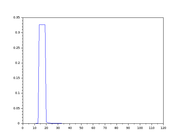
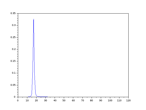
With the tracking resonators, each resonator if “attracted” by the closest and the strongest frequency peak. With a sound composed by a pure sine wave for example, several closest resonators will have their frequencies become close to the pure sine frequency. Each of these resonators will have almost the same value as shown in Figure 1 A change has been made to the Resonate algorithm to limit the tracking range of each tracking resonator, so that they don’t overlap in frequency. With this modification, the result of a group of resonators close to frequency peaks are represented by a peak and not by a flat top as shown in Figure 2. This eases the peak detection step we use after to compute the Color.
3.2 Use of smooth changes for resynthesis
The Resonate algorithm source code also provides an implementation of complex oscillators. They
provide a convenient and optimized way to resynthesize a sound from the frequency domain to
the temporal domain. This implementation has been slightly modified, by updating the
oscillators amplitudes and frequencies smoothly, with the same smooting  coefficient value
used for the resonators. This change prevents temporal domain sound discontinuities, that
would have produced audio clicks, without needing to handle this in any other parts of the
implementation.
4 The SAS model
The SAS model [1] is represented by the following parameters: Amplitude, Frequency, Color and Warping. Amplitude, Color and Warping are implemented as described in [1], taking as input the result of a tracking resonator bank. The Frequency parameter, or pitch, more complex to compute in a robust manner. For this purpose, we implemented a new method based on chroma domain transformation.
4.1 Chroma domain pitch finding
The frequency domain used in sound processing is often in the range corresponding to the average
human perception (20Hz to 20000Hz). We can convert any frequency from this domain to a chroma
value i.e. convert it to values in the normalized range from the musical notes C to B for example, with
all the intermediate values between notes in a continuous manner. We then optain an array of
amplitudes for each chroma value. The algorithm for computing the chroma array is described below 1.
It uses the MIDI note  as a base frequency and uses the following formula for the
backward computation
 . We use the same formula for getting the base
frequency from the main chroma peak. For getting the best octave from the result base frequency we
use the algorithm below 3.
(see Figure 3)
2: Get the chroma value for each resonator.
This is done in a backward manner:
for each chroma bin, retrieve the interpolated amplitude from the 2 closest resonators amplitudes.
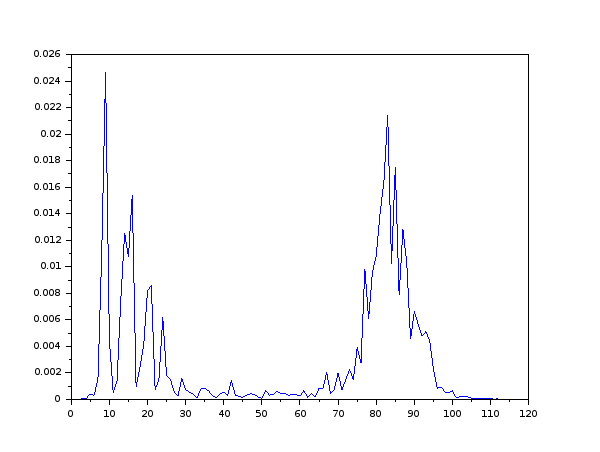
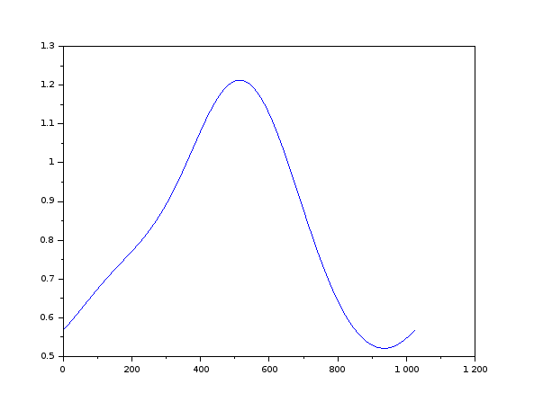
We obtain a curve with peaks corresponding the dominant chroma values (see Figure 4)
3: Smooth the chroma values.
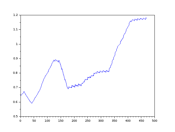
A smooting in the chroma domain is done on the values, so that one dominant peak emerges.
A temporal domain smoothing is also done (see Figure 5)
4: Find the main peak (maximum of the amplitudes in the chroma domain)
5: Make the inverse transformation, from chroma to frequency,
to get the base frequency corresponding to this main chroma peak
2: With the following score computation :
for the current octave candidate, sum the ponderated amplitudes of each harmonic,
with

4.1.1 Pitch finding algorithm results
This algorithm is robust and easy to implement and it handles the missing fundamental case. It has been tested on several types of sounds good results. There are however some cases where it fails at finding the right octave.
4.2 Implementation of a noise parameter for the SAS model
It is interesting to add a noise parameter to the SAS model, to be able to analyze and resynthesize the noisy parts of the signal (for example the breath in a vocal sound). For this we have used a simple but efficient method, by computing the spectral flatness of the input signal, and resynthesizing the noise in the temporal domain by using an inverse FFT transform.
4.2.1 Analysis of the noise
We take the result of the resonators, and compute the spectral flatness over it using the formula described in [4]. We obtain a noisiness array, similar to the Color and Warping ones 3

2: Compute the spectral flatness for each frequency by taking the neighbor amplitude
values inside a weighting window
4.2.2 Resynthesis of the noise
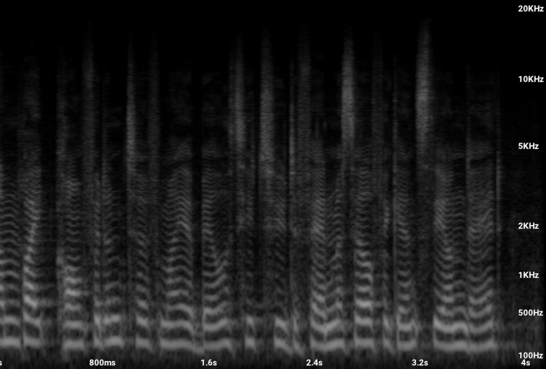
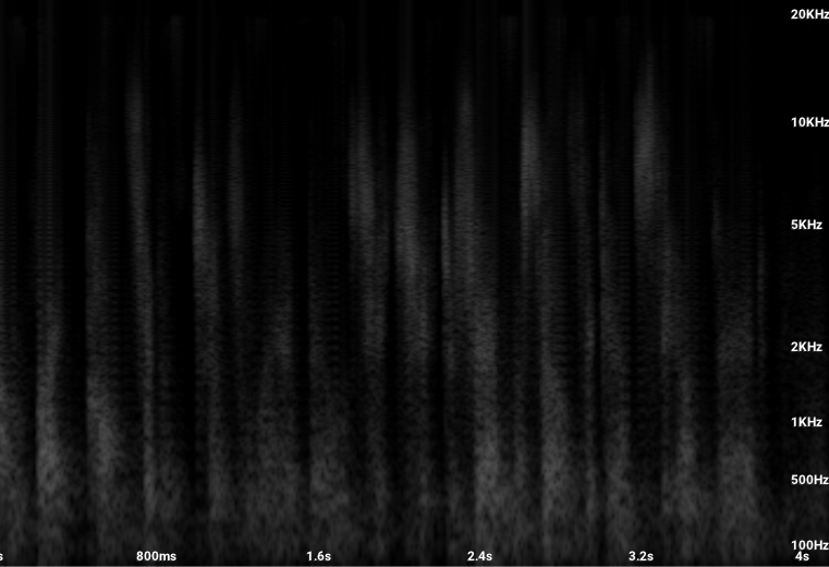
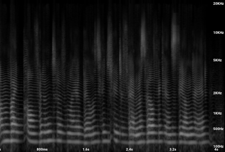
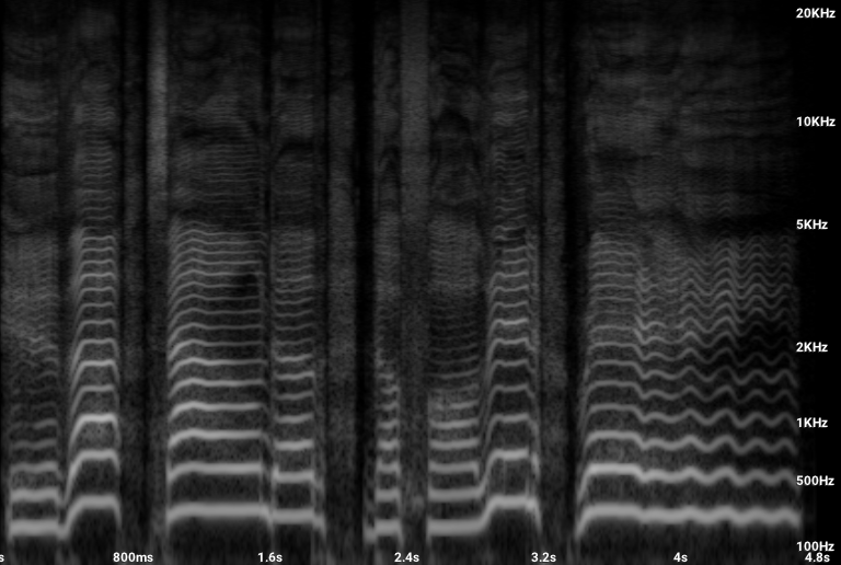
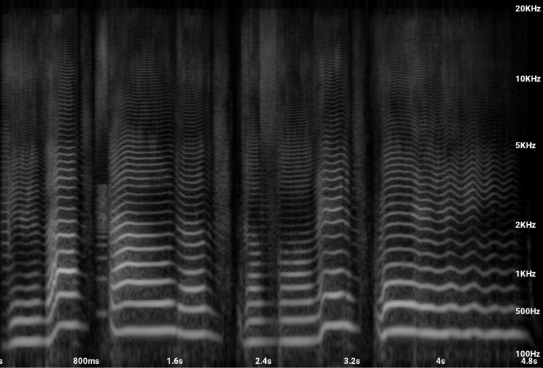
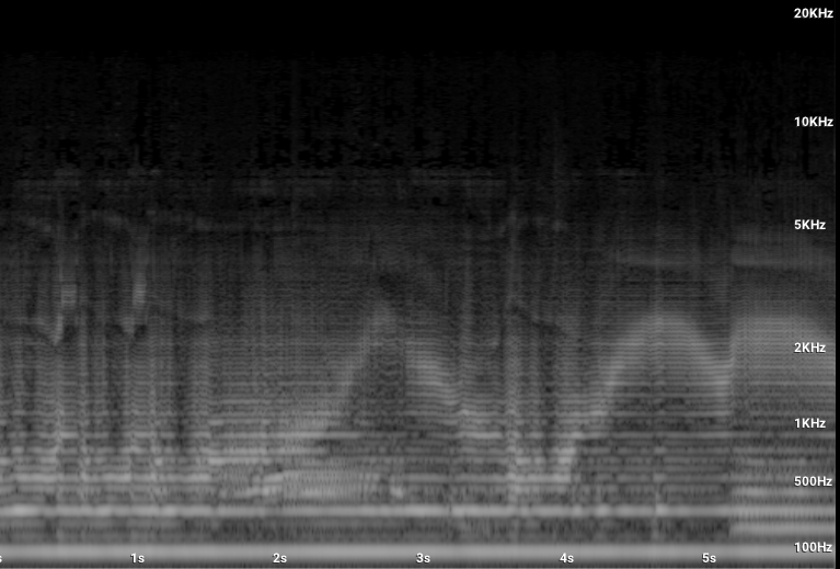
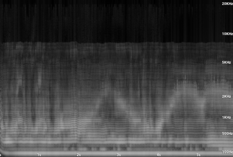
For resynthesizing the noise, we compute the inverse FFT of the spectral flatness array, which gives a temporal version of the noise part of the analyzed sound, that can be added to the result temporal domain signal. We adjust the ratio of the Harmonic Color and the Noise Color for each resynthesis oscillator and sample. The results can be seen in the spectrograms below 6 7 8.
4.3 Pitching the Color
We have made some pitch shifting tests and found interesting to also pitch the Color parameter of the SAS model.
5 Implementation notes
112 resonators have been used, with frequencies spread over a mel scale. This corresponds to an interval of one semi-tone between each resonator for a range between 20Hz and 2000Hz as described in [2]. For most of the tested sounds (singing voice and speaking voice for example), we keep this frequency range from 20 Hz to 20000 Hz. For some few others (for example a bass guitar sound), we use a frequency range from 1Hz to 2000Hz which increases the analysis resolution for the low frequencies. For the chroma array, we use a size of 1024 chroma bins, with a smooting Hann window of size 512. We use a SAS frame size of 112, and a temporal noise buffer size of 256. We compute a new SAS frame and update the synthesis parameters every 256 samples at a sampling rate of 44100Hz. In initialization of the synthesis phase, we put random phase values for the oscillators bank for preventing from DC offset effect that can occur if all the oscillator phases are set to the same value at initialization. The source code corresponding to this work is available at http://humble-nibble.org/sas-resonate.htm
6 Results
We implemented several LV2 plugins to test and use our simplementation, such a SAS analysis+resynthesis plugin. We also implemented a pair of plugins, the first one for converting single pitch harmonic sounds to MIDI, and another one to synthetize sounds from samples, taking MIDI as input. These plugins work with low latency and can be used in real-time.
6.1 Quality and performances
We have not made many comparisons, but our method gives good quality results, except when there are octave jumps. This method works with low latency (it handles latency of 256 samples at 44100Hz in our tests), and this latency can be decreased if we have the possibility to have a more powerful CPU. The plugins take around 25% of the CPU resources on a 8 cores standard computer. Examples can be found below 9 10 11 12.
7 Conclusion
We have developed an implementation of the SAS model using the Resonate algorithm. The current results look promizing, in term of quality and and in term of possibilities of use, even if there remains some artifacts in some cases. The current implementation can be used but under certain conditions.
References
[1] M. Desainte-Catherine, Sylvain Marchand. Structured Additive Synthesis: Towards a Model of Sound Timbre and Electroacoustic Music Forms. Proceedings of the International Computer Music Conference (ICMC99), Oct 1999, Beijing (CN), China. pp.260–263. 〈hal-00308406〉
[2] Alexandre R.J. François, “Resonate: Efficient Low Latency Spectral Analysis of Audio Signals,” in Proceedings of the 50th Anniversary of the International Computer Music Conference 2025, pp. 251-258, Boston, MA, USA, 8-14 June 2025.
[3] Alexandre R.J. François, “Real-Time, Low-Latency, High Resolution Audio Spectral Analysis: Phase Matters,” in Proceedings of the International Computer Music Conference 2026, pp. 150-157, Hamburg, Germany, 10-16 May 2026.
[4] G. Peeters. A Large Set of Audio Features for Sound Description (Similarity and Classification) in the CUIDADO Project. Cuidado Project Report, IRCAM, 2004. http://recherche.ircam.fr/anasyn/peeters/ARTICLES/Peeters_2003_cuidadoaudiofeatures.pdf
------------------------------------
pdf version of this page
source code